Critical points for various fluids
Code: #113-000
File: apps/van_der_waals/critical_points.ipynb
Run it online: ![]()
The aim of this notebook is to visualize the critical points of various fluids.
Interface
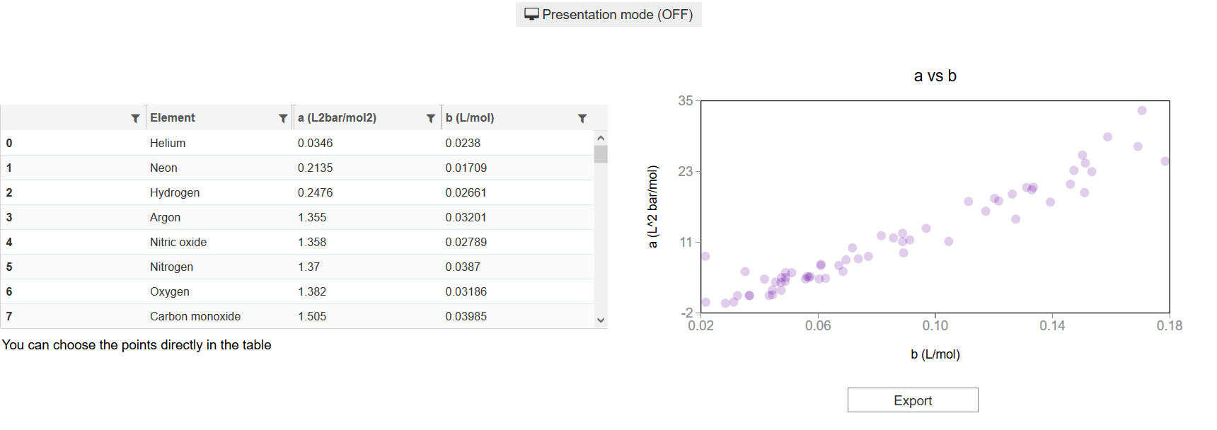
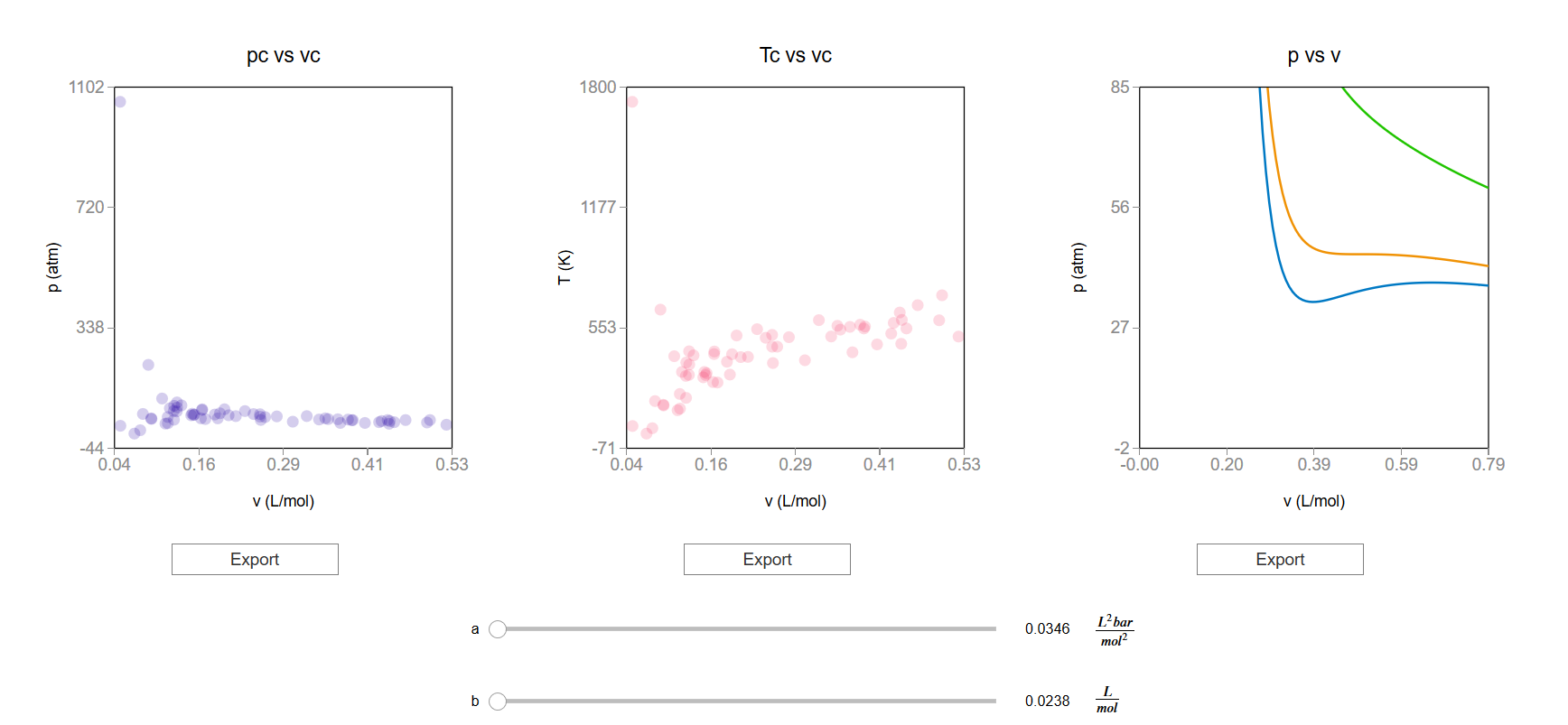
The main interface (main_block_113_000) is divided in three VBox: top_block_113_000, middle_block_113_000 and bottom_block_113_000. top_block_113_000 contains a bqplot Figure (fig_113_001) and a qgrid chart (qgrid_table). middle_block_113_000 contains of 3 bqplot Figures: fig_113_002, fig_113_003 and fig_113_005.
[1]:
from IPython.display import Image
Image(filename='../../static/images/apps/113-000_1.png')
[1]:
[2]:
Image(filename='../../static/images/apps/113-000_2.png')
[2]:
CSS
A custom css file is used to improve the interface of this application. It can be found here.
[1]:
from IPython.display import HTML
display(HTML("<head><link rel='stylesheet' type='text/css' href='./../../static/custom.css'></head>"))
display(HTML("<style>.container { width:100% !important; }</style>"))
Packages
[2]:
from bqplot import *
import bqplot as bq
import bqplot.marks as bqm
import bqplot.scales as bqs
import bqplot.axes as bqa

import ipywidgets as widgets

import scipy

import qgrid
import pandas as pd

import urllib.parse
import webbrowser

import sys
Physical functions
This are the functions that have a physical meaning:
calculate_criticget_absolute_isothermsbar_to_atm
[3]:
def calculate_critic(a, b):

    """
        This function calculates the critic point
        (p_c, v_c, T_c) from given a and b parameters of
        the Van der Waals equation of state for real gases.

        :math:`(P + a \\frac{n^2}{V^2})(V - nb) = nRT`

        :math:`p_c = \\frac{a}{27 b^2}`
        :math:`v_c = 3b`
        :math:`T_c = \\frac{8a}{27 b R}`

   Args:
       a: Term related with the attraction between particles in
       L^2 bar/mol^2.\n
       b: Term related with the volume that is occupied by one
       mole of the molecules in L/mol.\n

   Returns:
       p_c: Critical pressure in bar.\n
       v_c: Critical volume in L/mol.\n
       T_c: Critical tenperature in K.\n

    """

    if b == 0.0:
        return None

    k_B = 1.3806488e-23 #m^2 kg s^-2 K^-1
    N_A = 6.02214129e23
    R = 0.082 * 1.01325 #bar L mol^-1 K^-1

    p_c = a/27.0/(b**2)
    v_c = 3.0*b
    T_c = 8.0*a/27.0/b/R

    return p_c, v_c, T_c
[4]:
def get_absolute_isotherms(a, b, v_values, T_values):
    """This function calculates the theoretical p(v, T) plane
        (in absolute coordinates) according to van der Waals
        equation of state from a given range of volumes
        and tenperatures.

    Args:
        a: Term related with the attraction between particles in
           L^2 bar/mol^2.\n
        b: Term related with the volume that is occupied by one
        mole of the molecules in L/mol.\n
        v_values: An array containing the values of v
        for which the isotherms must be calculated.\n
        T_values: An array containing the values of T for which
        the isotherms must be calculated.\n


    Returns:
        isotherms: A list consisted of numpy arrays containing the
        pressures of each isotherm.
    """
    isotherms = []

    R = 0.082 * 1.01325 #bar L mol^-1 K^-1

    for T in T_values:

        isot = []

        for v in v_values:

            p = R*T/(v - b) - (a/v**2)
            isot = np.append(isot, p)

        isotherms.append(isot)

    return isotherms
[5]:
def bar_to_atm(p_values):
    """This function changes the pressures of an array
    form bars to atm.

    Args:
        p_values: List consisted of pressures in bars.\n

    Returns:
        p_values: List consisted of pressures in atm.\n
    """

    p_values = np.array(p_values) * 0.9869

    return p_values
[6]:
def generate_critical_points(df):
    """This function takes a Pandas dataframe containing three
    columns (element, a, b) and returns four lists: pc, vc, Tc and names

    Args:
        df: Pandas dataframe consisted of three columns: element, a, b.\n

    Returns:
        pc: A numpy array consisted of the values of the critical pressures.\n
        vc: A numpy array consisted of the values of the critical volumes.\n
        Tc: A numpy array consisted of the values of the critical tenperatures.\n
        names: A list consisted of the names of the elements.\n
    """

    pc = []
    vc = []
    Tc = []

    names = []

    name_values = df.iloc[:,0]
    a_values, b_values, names_sorted = get_a_b_names(df)

    for i in range(len(a_values)):

        names.append(names_sorted[i])

        a = float(a_values[i])
        b = float(b_values[i])
        p, v, T = calculate_critic(a, b)

        pc = np.append(pc, p)
        vc = np.append(vc, v)
        Tc = np.append(Tc, T)

    return pc, vc, Tc, names
[7]:
def get_a_b_names(df):
    """This function takes a pandas dataframe containing the
    columns 'a (L2bar/mol2)', 'b (L/mol)' and 'Element' and return the
    lists of the colums sorted by the values of 'a (L2bar/mol2)'.

    Args:
        df: Pandas dataframe consisted of three columns: 'a (L2bar/mol2)',
        'b (L/mol)' and 'Element'.\n

    Returns:
        a_values_sorted: A list array consisted of the sorted values of 'a (L2bar/mol2)'.\n
        b_values_sorted: A list array consisted of the sorted values of 'b (L/mol)'.\n
        names_sorted: A list consisted of the names of the sorted values of 'Element'.\n
    """

    a_values = list(df['a (L2bar/mol2)'])
    b_values = list(df['b (L/mol)'])
    names = list(df['Element'])

    a_values_sorted = sorted(a_values)

    #Sort values of b depending on the order of a
    b_values_sorted = [y for _,y in sorted(zip(a_values, b_values))]
    names_sorted = [y for _,y in sorted(zip(a_values, names))]

    return a_values_sorted, b_values_sorted, names_sorted
Main interface
[17]:
#data taken from https://en.wikipedia.org/wiki/Van_der_Waals_constants_(data_page) using https://wikitable2csv.ggor.de/
#format: Element, a (L2bar/mol2), b (L/mol)

raw_data = [
"Acetic acid",17.71,0.1065,
"Acetic anhydride",20.158,0.1263,
"Acetone",16.02,0.1124,
"Acetonitrile",17.81,0.1168,
"Acetylene",4.516,0.0522,
"Ammonia",4.225,0.0371,
"Argon",1.355,0.03201,
"Benzene",18.24,0.1154,
"Bromobenzene",28.94,0.1539,
"Butane",14.66,0.1226,
"Carbon dioxide",3.640,0.04267,
"Carbon disulfide",11.77,0.07685,
"Carbon monoxide",1.505,0.03985,
"Carbon tetrachloride",19.7483,0.1281,
"Chlorine",6.579,0.05622,
"Chlorobenzene",25.77,0.1453,
"Chloroethane",11.05,0.08651,
"Chloromethane",7.570,0.06483,
"Cyanogen",7.769,0.06901,
"Cyclohexane",23.11,0.1424,
"Diethyl ether",17.61,0.1344,
"Diethyl sulfide",19.00,0.1214,
"Dimethyl ether",8.180,0.07246,
"Dimethyl sulfide",13.04,0.09213,
"Ethane",5.562,0.0638,
"Ethanethiol",11.39,0.08098,
"Ethanol",12.18,0.08407,
"Ethyl acetate",20.72,0.1412,
"Ethylamine",10.74,0.08409,
"Fluorobenzene",20.19,0.1286,
"Fluoromethane",4.692,0.05264,
"Freon",10.78,0.0998,
"Germanium tetrachloride",22.90,0.1485,
"Helium",0.0346,0.0238,
"Hexane",24.71,0.1735,
"Hydrogen",0.2476,0.02661,
"Hydrogen bromide",4.510,0.04431,
"Hydrogen chloride",3.716,0.04081,
"Hydrogen selenide",5.338,0.04637,
"Hydrogen sulfide",4.490,0.04287,
"Iodobenzene",33.52,0.1656,
"Krypton",2.349,0.03978,
"Mercury",8.200,0.01696,
"Methane",2.283,0.04278,
"Methanol",9.649,0.06702,
"Neon",0.2135,0.01709,
"Nitric oxide",1.358,0.02789,
"Nitrogen",1.370,0.0387,
"Nitrogen dioxide",5.354,0.04424,
"Nitrous oxide",3.832,0.04415,
"Oxygen",1.382,0.03186,
"Pentane",19.26,0.146,
"Phosphine",4.692,0.05156,
"Propane",8.779,0.08445,
"Radon",6.601,0.06239,
"Silane",4.377,0.05786,
"Silicon tetrafluoride",4.251,0.05571,
"Sulfur dioxide",6.803,0.05636,
"Tin tetrachloride",27.27,0.1642,
"Toluene",24.38,0.1463,
"Water",5.536,0.03049,
"Xenon",4.250,0.05105
]
[ ]:
"""

.. module:: critical_points.ipynb
    :sypnopsis: This module creates an interface to interact with the
    critical points of different fluids.\n

.. moduleauthor:: Jon Gabirondo López (jgabirondo001@ikasle.ehu.eus)

"""

# Prepare the database

data_array = np.array(raw_data)
data_reshaped = np.reshape(data_array, (-1,3)); #reshape in three columns

database = pd.DataFrame(
    data=data_reshaped,
    columns=["Element", "a (L2bar/mol2)", "b (L/mol)"]
)

# numpy converts all elements to 'object' and
# pandas interprets them as string, but I want a and b values to be float
database["a (L2bar/mol2)"] = np.round(
    pd.to_numeric(database["a (L2bar/mol2)"]),
    4
)

database["b (L/mol)"] = np.round(
    pd.to_numeric(database["b (L/mol)"]),
    5
)

a_values, b_values, names_sorted = get_a_b_names(database)

database["Element"] = names_sorted
database["a (L2bar/mol2)"] = a_values
database["b (L/mol)"] = b_values

# Show the database in QGrid chart.

grid_options = {
    # SlickGrid options
    'fullWidthRows': True,
    'syncColumnCellResize': True,
    'forceFitColumns': True,
    'defaultColumnWidth': 150,
    'rowHeight': 28,
    'enableColumnReorder': False,
    'enableTextSelectionOnCells': True,
    'editable': False, #lehen True
    'autoEdit': False,
    'explicitInitialization': True,

    # Qgrid options
    'maxVisibleRows': 7, #we have changed it to 5 (default = 15)
    'minVisibleRows': 7, #we have changed it to 5 (default = 8)
    'sortable': True,
    'filterable': True,
    'highlightSelectedCell': False,
    'highlightSelectedRow': True
}

qgrid_table = qgrid.show_grid(database, grid_options=grid_options)

qgrid_table.on(['filter_changed'], change_visible_points)
qgrid_table.on(['selection_changed'], change_selected_points)

# QGrid triggering actions
#[
#    'cell_edited',
#    'selection_changed',
#    'viewport_changed',
#    'row_added',
#    'row_removed',
#    'filter_dropdown_shown',
#    'filter_changed',
#    'sort_changed',
#    'text_filter_viewport_changed',
#    'json_updated'
#]

########################################
###########TOP BLOCK####################
########################################

top_block_113_000 = widgets.VBox(
    [],
    layout=widgets.Layout(
        width='100%',
        align_self='center',
    )
)

fig_113_004 = bq.Figure(
    title='a vs b',
    marks=[],
    axes=[],
    animation_duration=0,
    legend_location='top-right',
    background_style= {'fill': 'white',  'stroke': 'black'},
    fig_margin=dict(top=80, bottom=80, left=80, right=30),
    toolbar = True,
    layout = widgets.Layout(height='400px')
)

scale_x_004 = bqs.LinearScale(min = min(b_values), max = max(b_values))
scale_y_004 = bqs.LinearScale(min = min(a_values), max = max(a_values))

axis_x_004 = bqa.Axis(
    scale=scale_x_004,
    tick_format='.2f',
    tick_style={'font-size': '15px'},
    num_ticks=5,
    grid_lines = 'none',
    grid_color = '#8e8e8e',
    label='b (L/mol)',
    label_location='middle',
    label_style={'stroke': 'black', 'default-size': 35},
    label_offset='50px'
)

axis_y_004 = bqa.Axis(
    scale=scale_y_004,
    tick_format='.0f',
    tick_style={'font-size': '15px'},
    num_ticks=4,
    grid_lines = 'none',
    grid_color = '#8e8e8e',
    orientation='vertical',
    label='a (L^2 bar/mol)',
    label_location='middle',
    label_style={'stroke': 'red', 'default_size': 35},
    label_offset='50px'
)

fig_113_004.axes = [axis_x_004, axis_y_004]

scatter_113_004 = bqm.Scatter(
    name = '',
    x = b_values,
    y = a_values,
    scales = {'x': scale_x_004, 'y': scale_y_004},
    default_opacities = [0.2],
    visible = True,
    colors = ['#6a03a1'],
    names = names_sorted,
    display_names = False,
    labels=[],
    tooltip = tt
)

scatter_113_004.on_hover(hover_handler)

fig_113_004.marks = [scatter_113_004]

message1 = widgets.HTML(value='<p>You can choose the points directly in the table</p>')

change_view_button = widgets.ToggleButton(
    value=False,
    description='Presentation mode (OFF)',
    disabled=False,
    button_style='',
    tooltip='',
    icon='desktop',
    layout=widgets.Layout(
        width='initial',
        align_self='center'
    )
)

change_view_button.observe(change_view, 'value')

prepare_export_fig_113_004_button = widgets.Button(
    description='Export',
    disabled=False,
    button_style='',
    tooltip='',
)

prepare_export_fig_113_004_button.on_click(prepare_export)

top_block_113_000.children = [
    change_view_button,
    widgets.HBox([
        widgets.VBox([
            qgrid_table,
            message1
        ],
            layout=widgets.Layout(
                width='50%',
                margin='80px 0 0 0'
            )
        ),
        widgets.VBox([
            fig_113_004,
            prepare_export_fig_113_004_button
        ],
            layout=widgets.Layout(
                width='50%',
                align_items='center',
            )
        )
    ])
]


########################################
###########MIDDLE BLOCK#################
########################################

middle_block_113_000 = widgets.HBox(
    [],
    layout=widgets.Layout(
        width='100%',
        align_self='center',
        align_content='center'
    )
)

fig_113_002 = bq.Figure(
    title='pc vs vc',
    marks=[],
    axes=[],
    animation_duration=0,
    legend_location='top-right',
    background_style= {'fill': 'white',  'stroke': 'black'},
    fig_margin=dict(top=80, bottom=80, left=80, right=30),
    toolbar = True,
    layout = widgets.Layout(width='90%')
)

fig_113_003 = bq.Figure(
    title='Tc vs vc',
    marks=[],
    axes=[],
    animation_duration=0,
    legend_location='top-right',
    background_style= {'fill': 'white',  'stroke': 'black'},
    fig_margin=dict(top=80, bottom=80, left=80, right=30),
    toolbar = True,
    layout = widgets.Layout(width='90%')
)


pc, vc, Tc, names = generate_critical_points(database)

scale_x_v = bqs.LinearScale(min = min(vc), max = max(vc))
scale_y_p = bqs.LinearScale(min = min(pc), max = max(pc))
scale_y_T = bqs.LinearScale(min = min(Tc), max = max(Tc))


axis_x_v = bqa.Axis(
    scale=scale_x_v,
    tick_format='.2f',
    tick_style={'font-size': '15px'},
    num_ticks=5,
    grid_lines = 'none',
    grid_color = '#8e8e8e',
    label='v (L/mol)',
    label_location='middle',
    label_style={'stroke': 'black', 'default-size': 35},
    label_offset='50px'
)

axis_y_p = bqa.Axis(
    scale=scale_y_p,
    tick_format='.0f',#'0.2f',
    tick_style={'font-size': '15px'},
    num_ticks=4,
    grid_lines = 'none',
    grid_color = '#8e8e8e',
    orientation='vertical',
    label='p (atm)',
    label_location='middle',
    label_style={'stroke': 'red', 'default_size': 35},
    label_offset='50px'
)

axis_y_T = bqa.Axis(
    scale=scale_y_T,
    tick_format='.0f',#'0.2f',
    tick_style={'font-size': '15px'},
    num_ticks=4,
    grid_lines = 'none',
    grid_color = '#8e8e8e',
    orientation='vertical',
    label='T (K)',
    label_location='middle',
    label_style={'stroke': 'red', 'default_size': 35},
    label_offset='50px'
)


fig_113_002.axes = [axis_x_v, axis_y_p]
fig_113_003.axes = [axis_x_v, axis_y_T]

scatter_113_002 = bqm.Scatter(
    name = '',
    x = vc,
    y = pc,
    scales = {'x': scale_x_v, 'y': scale_y_p},
    default_opacities = [0.2],
    visible = True,
    colors = ['#2807a3'],
    names = names,
    display_names = False,
    labels=[],
    tooltip = tt
)

scatter_113_002.on_hover(hover_handler)

scatter_113_003 = bqm.Scatter(
    name = '',
    x = vc,
    y = Tc,
    scales = {'x': scale_x_v, 'y': scale_y_T},
    default_opacities = [0.2 for v in vc],
    visible = True,
    colors = ['#f5426c'],
    names = names,
    display_names = False,
    labels=[],
    tooltip = tt
)

scatter_113_003.on_hover(hover_handler)


tracer_113_002 = bqm.Scatter(
    name = 'tracer_113_002',
    x = [1.0],
    y = [1.0],
    scales = {'x': scale_x_v, 'y': scale_y_p},
    default_opacities = [1.0],
    visible = True,
    colors=['black'],
)

tracer_113_003 = bqm.Scatter(
    name = 'tracer_113_003',
    x = [1.0],
    y = [1.0],
    scales = {'x': scale_x_v, 'y': scale_y_T},
    default_opacities = [1.0],
    visible = True,
    colors=['black'],
)

selected_113_002 = bqm.Scatter(
    name = 'selected_113_002',
    x = [],
    y = [],
    scales = {'x': scale_x_v, 'y': scale_y_p},
    default_opacities = [1.0],
    visible = True,
    display_names = False,
    colors = scatter_113_002.colors,
    tooltip = tt
)

selected_113_002.on_hover(hover_handler)

selected_113_003 = bqm.Scatter(
    name = 'selected_113_003',
    x = [],
    y = [],
    scales = {'x': scale_x_v, 'y': scale_y_T},
    default_opacities = [1.0],
    visible = True,
    display_names = False,
    colors = scatter_113_003.colors,
    tooltip = tt
)

selected_113_002.on_hover(hover_handler)

fig_113_002.marks = [
    scatter_113_002,
    selected_113_002,
    tracer_113_002
]

fig_113_003.marks = [
    scatter_113_003,
    selected_113_003,
    tracer_113_003
]

colors = ['#0079c4','#f09205','#21c400']

fig_113_005 = bq.Figure(
    title='p vs v',
    marks=[],
    axes=[],
    animation_duration=500,
    legend_location='top-right',
    background_style= {'fill': 'white',  'stroke': 'black'},
    fig_margin=dict(top=80, bottom=80, left=80, right=20),
    toolbar = True,
    layout = widgets.Layout(width='90%')
)

p_values = []
v_values = []

for i in range(len(a_values)):

    a = a_values[i]
    b = b_values[i]


    p_c, v_c, T_c = calculate_critic(a, b)

    v = np.linspace(0.45*v_c, 5.0*v_c, 300)
    T_values = [0.95*T_c, T_c, 1.2*T_c]

    p = get_absolute_isotherms(a, b, v, T_values)

    p_values.append(bar_to_atm(p))
    v_values.append(v)

v_mean = np.mean(v_values)
v_min = np.min(v_values)

p_mean = np.mean(p_values)
p_min = np.min(p_values)

scale_x_005 = bqs.LinearScale(min = 0.0, max = 1.2*v_mean)
scale_y_005 = bqs.LinearScale(min = 0.0, max = 1.2*p_mean)

axis_x_005 = bqa.Axis(
    scale=scale_x_005,
    tick_format='.2f',
    tick_style={'font-size': '15px'},
    num_ticks=5,
    grid_lines = 'none',
    grid_color = '#8e8e8e',
    label='v (L/mol)',
    label_location='middle',
    label_style={'stroke': 'black', 'default-size': 35},
    label_offset='50px'
)


axis_y_005 = bqa.Axis(
    scale=scale_y_005,
    tick_format='.0f',
    tick_style={'font-size': '15px'},
    num_ticks=4,
    grid_lines = 'none',
    grid_color = '#8e8e8e',
    orientation='vertical',
    label='p (atm)',
    label_location='middle',
    label_style={'stroke': 'red', 'default_size': 35},
    label_offset='50px'
)

fig_113_005.axes = [axis_x_005, axis_y_005]

marks = []

for i in range(len(a_values)):

    marks.append(bqm.Lines(
        x = v_values[i],
        y = p_values[i],
        scales = {'x': scale_x_005, 'y': scale_y_005},
        opacities = [1.0 for elem in p_values],
        visible = a == a_values[i],
        colors = colors,
        labels = [names_sorted[i]]
        )
    )

fig_113_005.marks = marks

prepare_export_fig_113_002_button = widgets.Button(
        description='Export',
        disabled=False,
        button_style='',
        tooltip='',
    )

prepare_export_fig_113_002_button.on_click(prepare_export)

prepare_export_fig_113_003_button = widgets.Button(
        description='Export',
        disabled=False,
        button_style='',
        tooltip='',
    )

prepare_export_fig_113_003_button.on_click(prepare_export)

prepare_export_fig_113_005_button = widgets.Button(
        description='Export',
        disabled=False,
        button_style='',
        tooltip='',
    )

prepare_export_fig_113_005_button.on_click(prepare_export)

middle_block_113_000.children = [
    widgets.VBox([
        fig_113_002,
        prepare_export_fig_113_002_button
    ],
        layout=widgets.Layout(
            width='33%',
            align_items='center',
        )
    ),
    widgets.VBox([
        fig_113_003,
        prepare_export_fig_113_003_button
    ],
        layout=widgets.Layout(
            width='33%',
            align_items='center',
        )
    ),
    widgets.VBox([
        fig_113_005,
        prepare_export_fig_113_005_button
    ],
        layout=widgets.Layout(
            width='33%',
            align_items='center',
        )
    )
]

########################################
###########BOTTOM BLOCK#################
########################################
bottom_block_113_000 = widgets.VBox(
    [],
    layout=widgets.Layout(
        align_items='center',
        width='100%',
        margin='30px 0 0 0'
    )
)

a_slider = widgets.SelectionSlider(
    options=a_values,
    value=a_values[0],
    description='a',
    disabled=False,
    continuous_update=True,
    orientation='horizontal',
    readout=True,
    layout=widgets.Layout(width='90%'),
)

a_slider.observe(update_sliders, 'value')

b_slider = widgets.SelectionSlider(
    options=b_values,
    value=b_values[0],
    description='b',
    disabled=False,
    continuous_update=True,
    orientation='horizontal',
    readout=True,
    layout=widgets.Layout(width='90%'),
)

b_slider.observe(update_sliders, 'value')

bottom_block_113_000.children = [
    widgets.HBox([
        a_slider,
        widgets.HTMLMath(
            value=r"\( \frac{L^2 bar}{mol^2} \)",
            layout=widgets.Layout(height='60px')
        )],
        layout=widgets.Layout(
            width='50%',
            height='100%'
        )
    ),
    widgets.HBox([
        b_slider,
        widgets.HTMLMath(
            value=r"\( \frac{L}{mol} \)",
            layout=widgets.Layout(height='60px')
        )],
        layout=widgets.Layout(width='50%', height='100%')
    )
]

########################################
###########MAIN BLOCK###################
########################################

main_block_113_000 = widgets.VBox(
    [],
    layout=widgets.Layout(align_content='center')
)

main_block_113_000.children = [
    top_block_113_000,
    middle_block_113_000,
    bottom_block_113_000
]

figures = [
    fig_113_002,
    fig_113_003,
    fig_113_004,
    fig_113_005
]

main_block_113_000